Interest Accrual

In our original design, the relationship between where interest is accrued and where it is distributed is a bit tricky since market making liquidity can be borrowed and the individual assets are also lent out. This is because most of these individual assets are not used in an AMM with Uniswap V2 type liquidity. Here is a drawing showing where X, Y, and K are being borrowed from.

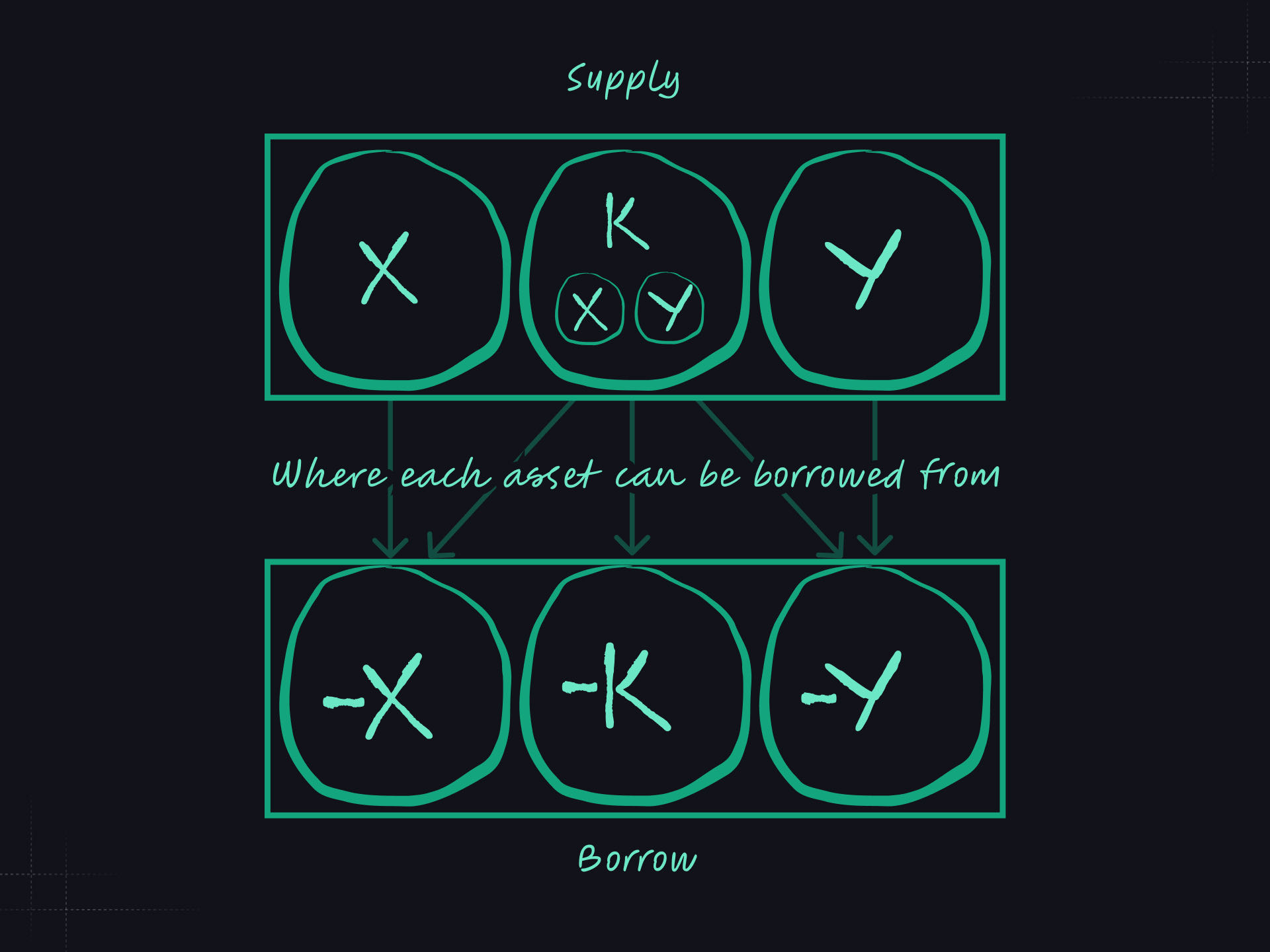
Borrowed $X$ and $Y$

Borrowed $X$ and $Y$ are distributed pro rata between the depositors of $X$ and $K$ as well as $Y$ and $K$. Since the quantity of $X$ and $Y$ that make up $K$ fluctuates with the change of price, the geometric mean between state updates is used to determine how much was available of each to be borrowed between two given state updates. Using the geometric mean reduces the impact of outliers and thus minimizes the potency of someone trying to modify the price before a state update to earn a larger pro rata share of accrued interest.

Borrowed $K$

When borrowing liquidity, first we consider the total deposited $K$, then subtract the borrowed $K$ to determine how much liquidity is active and available. It is important to note that the accounting for this borrowed liquidity is not done in units of $K$, but rather in liquidity, $L$, such that $L=\sqrt{K}$. The difference between total liquidity and the borrowed liquidity is called activeLiquidity. The active liquidity is what is available for both swaps, and to be borrowed individually in the form of $X$ and $Y$. This means that borrowed $X$ and $Y$ will eat into the available liquidity that can be borrowed in the form of $K$ and vice versa.

Utilization based Rates

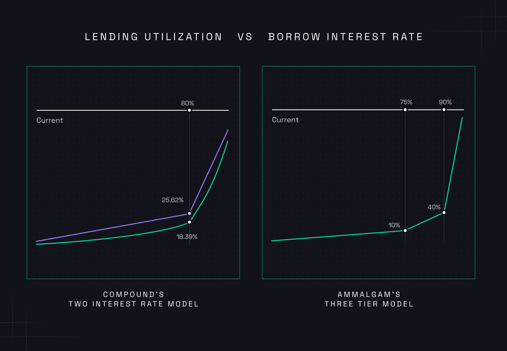
We use a slightly modified version of the two tier utilization model used by Compound and Aave. We want to emulate the sweet spot property of these models that lower lending rates prior to the sweet spot to encourage increased utilization and then increase aggressively after to encourage enough liquidity to allow for withdrawals. We add a third transition between when the max borrow is achieved at 90% utilization of $X$ and $Y$ and the depletion of asset that changes the invariant curve kick in at 95% utilization. This increases rates even faster to magnify incentivize to pay down debts or attract additional liquidity when an asset is depleted. See Three Tier Lending Utilization Rate Increase section of the depleted asset protection for more details.

If 40% yield rates are still not bringing liquidity back to the pair, the market is really starting to unwind. At this stage the FUD is catching on and there may even be enough market momentum to lead to cascading liquidations and forced selling. But, it's probably too early to call it a death spiral. The protocol has already stopped borrowing for the scarce asset, but more trades are taking it than bringing it. As these trades continue to take out liquidity, we introduce a third interest rate tier. Money market protocols use a two tier model. The first slowly increases rates as borrow utilization goes from 0% to some sweet spot, typically 80%. After this, rates start to increase faster between the sweet spot and 100% utilization. Our third tier allows for a third, more aggressive, rate increase once a reserve's health is at risk. Now each trade taking liquidity is noticeably raising interest rates further increasing the pain of borrowing and enticing what would be otherwise bystanders to jump in with liquidity to yield farm the high rate. Once rates surpass 100, 200, 500% annualized, it is hard imagine the market not noticing and stepping in to relieve the pressure.

If this mechanism is still failing to stop the flow of liquidity out of the pair contract, the market is likely experiencing a death spiral. Interest rates might become completely meaningless. At this stage our mechanism design now needs to be ready for anything. The next response is designed to maintain sufficient liquidity to continue to fill swaps when no one is willing to provide liquidity or repay loans and the bountiful asset in the contract is going to zero and the market is violently trying to secure as much of the scarce asset as it can.